Train a Machine Learning Model with Jupyter Notebook
Jupyter is a common web-based notebook for users to interactively write python programs together with documents. In our demo Spark cluster template, Jupyter has been pre-configured to connect to the Spark cluster.
In the following, we show how to use Jupyter to run a small machine job on Spark cluster interactively. Particularly, we’ll use Spark ML library to create a model to predict customer churn in a telecommunication company.
1. Open the Jupyter notebook.
Connect web browser to http://<masterIP>:8888 or click on the Jupyter Notebook link in the cluster info page as shown below.

Then, users will see the home page of Jupyter notebook few examples.
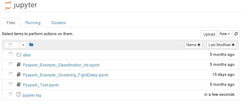
Users can create a new notebook, upload a notebook, or open a shell console.
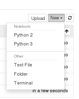
2. Download and copy sample dataset to HDFS.
First, open a shell console. Click New -> Terminal on the Jupyter home page.
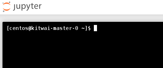
Then, execute the following shell commands.
wget https://github.com/kitwaicloud/kitwaicloud.github.io/raw/master/dataset/churn-bigml-80.csv
wget https://github.com/kitwaicloud/kitwaicloud.github.io/raw/master/dataset/churn-bigml-20.csv
hdfs dfs -mkdir dataset
hdfs dfs -put churn-bigml-80.csv dataset
hdfs dfs -put churn-bigml-20.csv dataset
Check the sample dataset in HDFS
hdfs dfs -ls dataset
Found 2 items
-rw-r--r--   1 centos supergroup      56329 2018-03-13 17:22 dataset/churn-bigml-20.csv
-rw-r--r--   1 centos supergroup     223998 2018-03-13 09:39 dataset/churn-bigml-80.csv
This dataset provides details of customers and labels if they cancel the subscription.
3. Create a new Python 3 notebook
Click on New -> Python 3.
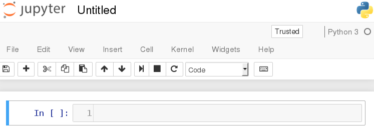
Then, we can start writing python code into Jupyter code cells. For each code cell, we can run it.
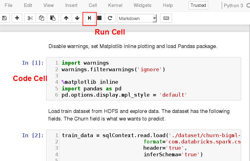
Next, we will train a machine learning model by a series of code blocks. Code and run each of them sequentially to gain interactive programming experience. Otherwise, the entire notebook can be downloaded from https://github.com/kitwaicloud/kitwaicloud.github.io/raw/master/jupyter/ChurnPrediction.ipynb
4. Load and explore data
Disable warnings, set Matplotlib inline plotting and load Pandas package.
import warnings
warnings.filterwarnings('ignore')

%matplotlib inline
import pandas as pd
#pd.options.display.mpl_style = 'default'    # mpl_style is deprecated
Load train dataset from HDFS and explore data. The dataset has the following fields. The Churn field is what we wants to predict.
train_data = sqlContext.read.load('./dataset/churn-bigml-80.csv',
                        format='com.databricks.spark.csv',
                        header='true',
                        inferSchema='true')

train_data.cache()
train_data.printSchema()
The output show that the dataset consists of 20 fields.
root
|-- State: string (nullable = true)
|-- Account length: integer (nullable = true)
|-- Area code: integer (nullable = true)
|-- International plan: string (nullable = true)
|-- Voice mail plan: string (nullable = true)
|-- Number vmail messages: integer (nullable = true)
|-- Total day minutes: double (nullable = true)
|-- Total day calls: integer (nullable = true)
|-- Total day charge: double (nullable = true)
|-- Total eve minutes: double (nullable = true)
|-- Total eve calls: integer (nullable = true)
|-- Total eve charge: double (nullable = true)
|-- Total night minutes: double (nullable = true)
|-- Total night calls: integer (nullable = true)
|-- Total night charge: double (nullable = true)
|-- Total intl minutes: double (nullable = true)
|-- Total intl calls: integer (nullable = true)
|-- Total intl charge: double (nullable = true)
|-- Customer service calls: integer (nullable = true)
|-- Churn: boolean (nullable = true)
Explore the first five rows.
pd.DataFrame(train_data.take(5), columns=train_data.columns)
| State | Account length | Area code | International plan | Voice mail plan | Number vmail messages | Total day minutes | Total day calls | Total day charge | Total eve minutes | Total eve calls | Total eve charge | Total night minutes | Total night calls | Total night charge | Total intl minutes | Total intl calls | Total intl charge | Customer service calls | Churn | |
|---|---|---|---|---|---|---|---|---|---|---|---|---|---|---|---|---|---|---|---|---|
| 0 | KS | 128 | 415 | No | Yes | 25 | 265.1 | 110 | 45.07 | 197.4 | 99 | 16.78 | 244.7 | 91 | 11.01 | 10.0 | 3 | 2.70 | 1 | False |
| 1 | OH | 107 | 415 | No | Yes | 26 | 161.6 | 123 | 27.47 | 195.5 | 103 | 16.62 | 254.4 | 103 | 11.45 | 13.7 | 3 | 3.70 | 1 | False |
| 2 | NJ | 137 | 415 | No | No | 0 | 243.4 | 114 | 41.38 | 121.2 | 110 | 10.30 | 162.6 | 104 | 7.32 | 12.2 | 5 | 3.29 | 0 | False |
| 3 | OH | 84 | 408 | Yes | No | 0 | 299.4 | 71 | 50.90 | 61.9 | 88 | 5.26 | 196.9 | 89 | 8.86 | 6.6 | 7 | 1.78 | 2 | False |
| 4 | OK | 75 | 415 | Yes | No | 0 | 166.7 | 113 | 28.34 | 148.3 | 122 | 12.61 | 186.9 | 121 | 8.41 | 10.1 | 3 | 2.73 | 3 | False |
Show summary statistics of all fields.
train_data.describe().toPandas()
| summary | State | Account length | Area code | International plan | Voice mail plan | Number vmail messages | Total day minutes | Total day calls | Total day charge | Total eve minutes | Total eve calls | Total eve charge | Total night minutes | Total night calls | Total night charge | Total intl minutes | Total intl calls | Total intl charge | Customer service calls | |
|---|---|---|---|---|---|---|---|---|---|---|---|---|---|---|---|---|---|---|---|---|
| 0 | count | 2666 | 2666 | 2666 | 2666 | 2666 | 2666 | 2666 | 2666 | 2666 | 2666 | 2666 | 2666 | 2666 | 2666 | 2666 | 2666 | 2666 | 2666 | 2666 |
| 1 | mean | None | 100.62040510127532 | 437.43885971492875 | None | None | 8.021755438859715 | 179.48162040510135 | 100.31020255063765 | 30.512404351087813 | 200.38615903976006 | 100.02363090772693 | 17.033072018004518 | 201.16894223555968 | 100.10615153788447 | 9.052689422355604 | 10.23702175543886 | 4.467366841710428 | 2.764489872468112 | 1.5626406601650413 |
| 2 | stddev | None | 39.56397365334985 | 42.521018019427174 | None | None | 13.61227701829193 | 54.21035022086982 | 19.988162186059512 | 9.215732907163497 | 50.95151511764598 | 20.16144511531889 | 4.330864176799864 | 50.780323368725206 | 19.418458551101697 | 2.2851195129157564 | 2.7883485770512566 | 2.4561949030129466 | 0.7528120531228477 | 1.3112357589949093 |
| 3 | min | AK | 1 | 408 | No | No | 0 | 0.0 | 0 | 0.0 | 0.0 | 0 | 0.0 | 43.7 | 33 | 1.97 | 0.0 | 0 | 0.0 | 0 |
| 4 | max | WY | 243 | 510 | Yes | Yes | 50 | 350.8 | 160 | 59.64 | 363.7 | 170 | 30.91 | 395.0 | 166 | 17.77 | 20.0 | 20 | 5.4 | 9 |
Count churn customers.
train_data.groupBy('Churn').count().show()
The output is as follows.
+-----+-----+
|Churn|count|
+-----+-----+
| true|  388|
|false| 2278|
+-----+-----+
5. Create a Logistic Regression model
Convert categorical fields into numeric fields.
from pyspark.ml.feature import StringIndexer
from pyspark.ml.feature import OneHotEncoder

ipIndexer = StringIndexer(inputCol = 'International plan', outputCol = 'ipIndex')
ipEncoder = OneHotEncoder(inputCol = 'ipIndex', outputCol = 'ipVector')
Define feature fields. We choose to ignore some fields as we think they are not relevant.
from pyspark.ml.feature import VectorAssembler

featureCols = ['Account length', 'ipVector', 'Number vmail messages', 'Total day minutes',
   'Total day calls', 'Total eve minutes', 'Total eve calls', 'Total night minutes', 'Total night calls',
   'Total intl minutes', 'Total intl calls', 'Customer service calls']
assembler = VectorAssembler(inputCols = featureCols, outputCol = 'features')
Create a logistic transformer.
from pyspark.ml.classification import LogisticRegression

lr = LogisticRegression(maxIter = 20)
Create numeric label field.
from pyspark.sql.types import DoubleType
from pyspark.sql.functions import udf

toNum = udf(lambda v: float(v), DoubleType())
train_data = train_data.withColumn('label', toNum(train_data['Churn'])).cache()
pd.DataFrame(train_data.take(5), columns=train_data.columns)
| State | Account length | Area code | International plan | Voice mail plan | Number vmail messages | Total day minutes | Total day calls | Total day charge | Total eve minutes | ... | Total eve charge | Total night minutes | Total night calls | Total night charge | Total intl minutes | Total intl calls | Total intl charge | Customer service calls | Churn | label | |
|---|---|---|---|---|---|---|---|---|---|---|---|---|---|---|---|---|---|---|---|---|---|
| 0 | KS | 128 | 415 | No | Yes | 25 | 265.1 | 110 | 45.07 | 197.4 | ... | 16.78 | 244.7 | 91 | 11.01 | 10.0 | 3 | 2.70 | 1 | False | 0.0 |
| 1 | OH | 107 | 415 | No | Yes | 26 | 161.6 | 123 | 27.47 | 195.5 | ... | 16.62 | 254.4 | 103 | 11.45 | 13.7 | 3 | 3.70 | 1 | False | 0.0 |
| 2 | NJ | 137 | 415 | No | No | 0 | 243.4 | 114 | 41.38 | 121.2 | ... | 10.30 | 162.6 | 104 | 7.32 | 12.2 | 5 | 3.29 | 0 | False | 0.0 |
| 3 | OH | 84 | 408 | Yes | No | 0 | 299.4 | 71 | 50.90 | 61.9 | ... | 5.26 | 196.9 | 89 | 8.86 | 6.6 | 7 | 1.78 | 2 | False | 0.0 |
| 4 | OK | 75 | 415 | Yes | No | 0 | 166.7 | 113 | 28.34 | 148.3 | ... | 12.61 | 186.9 | 121 | 8.41 | 10.1 | 3 | 2.73 | 3 | False | 0.0 |
5 rows × 21 columns
Chain all transformers and train the model.
from pyspark.ml import Pipeline

pipeline = Pipeline(stages=[ipIndexer, ipEncoder, assembler, lr])
model = pipeline.fit(train_data)
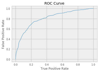
Display auROC of the trained model.
lrModel = model.stages[-1]
trainingSummary = lrModel.summary
print ('Train auROC = %3.2f' % trainingSummary.areaUnderROC)
Train auROC = 0.81
Plot ROC Curve.
import matplotlib.pyplot as plt

roc = trainingSummary.roc.toPandas()
plt.plot(roc['FPR'], roc['TPR'])
plt.ylabel('False Positive Rate')
plt.xlabel('True Positive Rate')
plt.title('ROC Curve')
plt.show()
6. Evaluate the model
Load test dataset from HDFS and evaluate the model with test data.
test_data = sqlContext.read.load('./dataset/churn-bigml-20.csv',
                        format='com.databricks.spark.csv',
                        header='true',
                        inferSchema='true')

test_data.cache()
test_data = test_data.withColumn('label', toNum(test_data['Churn'])).cache()

predictions = model.transform(test_data)
Evaluate the auROC of the test data.
from pyspark.ml.evaluation import BinaryClassificationEvaluator

evaluator = BinaryClassificationEvaluator(labelCol='label', rawPredictionCol='rawPrediction')
auROC = evaluator.evaluate(predictions)
print("Test auROC = %3.2f" % auROC)
Test auROC = 0.80
Evaluate the accuracy of the test data.
from pyspark.ml.evaluation import MulticlassClassificationEvaluator

multi = MulticlassClassificationEvaluator(labelCol='label', predictionCol='prediction', metricName="accuracy")
accuracy = multi.evaluate(predictions)
print("Accuracy = %3.2f" % accuracy)
Accuracy = 0.850075
Users can try to adjust training parameters to improve the accuracy of prediction.
7. Export the trained model for deployment
Export the model into PMML format. The PMML file can be downloaded and deployed with other tools such as Openscoring. Users can also deploy the PMML model with KitWai Openscoring cluster. See How to Deploy a Spark ML Model for more details.
from pyspark2pmml import PMMLBuilder
pmmlBytes = PMMLBuilder(sc, train_data, model).buildByteArray()

# Jpmml sparkml lib for python 2 is no longer supported.
#from jpmml_sparkml import toPMMLBytes
#pmmlBytes = toPMMLBytes(sc, train_data, model)

#print(pmmlBytes.decode("UTF-8"))

pmml = pmmlBytes.decode("UTF-8")
file = open("/tmp/churn.pmml","w")
file.write(pmml)
file.close()